Reducing Latency in Real-Time Speech Recognition: 2026 Guide

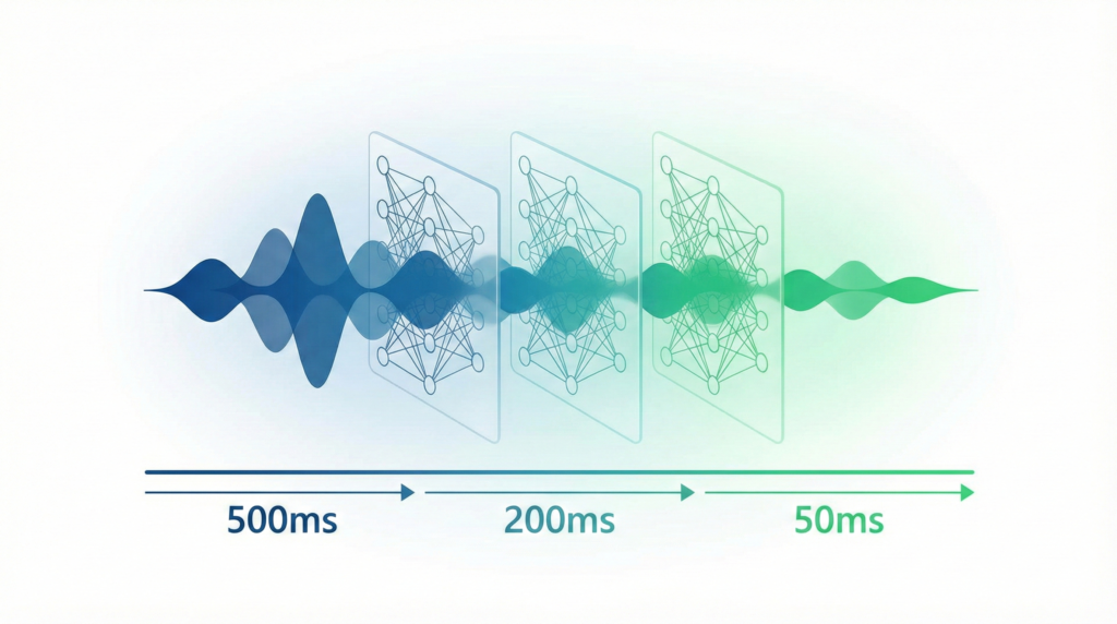
Real-time speech recognition has become essential for contact centres, healthcare documentation, and voice AI applications. However, achieving low-latency real-time speech recognition remains challenging, with many systems struggling to deliver transcripts in under 500 milliseconds. In this comprehensive guide, you’ll learn proven techniques to reduce latency in ASR systems, from architectural optimisations to hardware acceleration strategies that can transform your transcription performance.

What Causes Latency in Real-Time Speech Recognition?

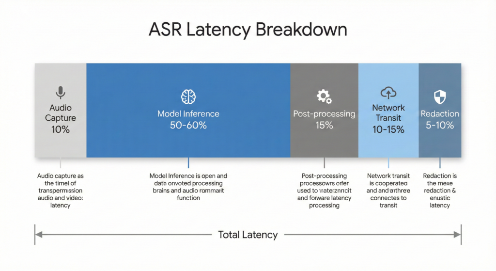
Understanding latency sources is crucial for optimisation. Total latency in real-time ASR systems stems from five primary components, with model inference accounting for 50-60% of the delay.

Audio capture and buffering introduces the first delay, typically 20-50 milliseconds depending on frame size. Smaller frames reduce latency but increase computational overhead, requiring careful balance for your specific use case.

Model inference dominates the latency budget. A vanilla Whisper large-v2 model can take 4-5 seconds to process just 13 minutes of audio on standard GPUs. This is where architectural optimisations and model compression deliver the most significant improvements.

Post-processing and formatting adds 50-100 milliseconds for punctuation, capitalisation, and entity formatting. Advanced systems now process these steps concurrently with model inference to reduce sequential delays.

Network transit time varies by geography and infrastructure, typically ranging from 50-200 milliseconds for cloud-based systems. Edge deployment can eliminate this entirely, though it introduces different trade-offs.

Compliance and redaction for sensitive data (PII, payment information) adds another 50-100 milliseconds but remains essential for healthcare and financial applications. You can’t skip this step in regulated industries, so optimising its implementation becomes critical.

How Do Streaming Architectures Reduce Latency?

Traditional ASR models process complete utterances, creating unnecessary delays for real-time applications. Streaming architectures fundamentally redesign how models consume and process audio, enabling progressive transcription as speech occurs.

Chunked Attention vs Causal Attention

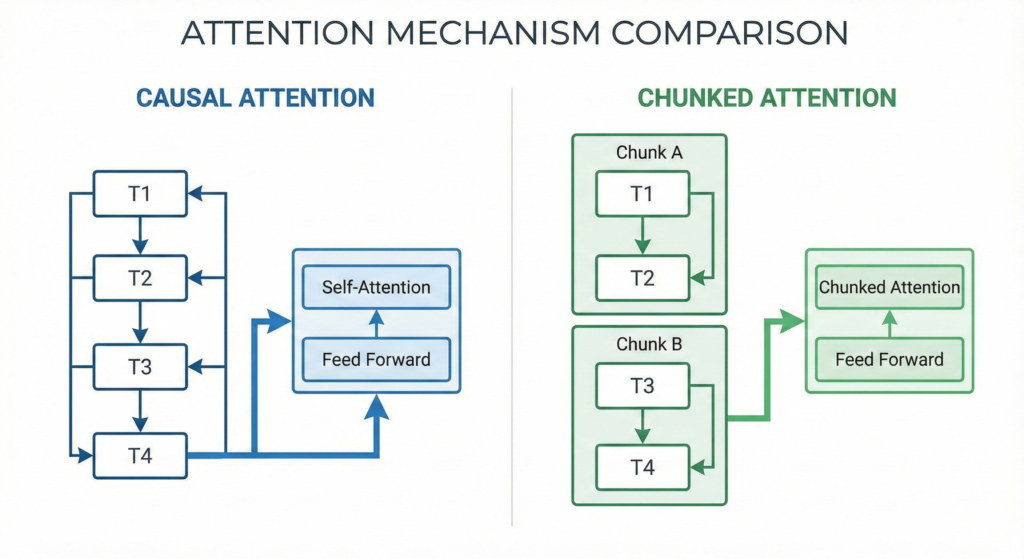
The choice between attention mechanisms significantly impacts both accuracy and latency. Causal attention is conceptually simple—each timestep only attends to current and past inputs. However, this severely degrades word error rates in practice.

Chunked attention offers a superior alternative. By grouping frames into fixed-size chunks (typically 16-32 frames) and allowing limited look-back context (40-50 frames), you maintain streaming capabilities whilst preserving accuracy. The SpeechBrain implementation demonstrates this approach effectively, achieving competitive WER with sub-200ms real-time factors.

Conformer-CTC Architecture for Streaming

Conformer models with Connectionist Temporal Classification have emerged as the dominant architecture for streaming speech recognition. Unlike attention-based models requiring full utterances, CTC enables frame-synchronous output suitable for streaming applications.

NVIDIA’s NeMo Conformer models achieve real-time factors below 0.2 on GPU, meaning they process 10 seconds of audio in just 2 seconds. This 5x speed advantage over real-time is crucial for handling concurrent streams in production environments.

For telecom and call centre applications, specialised Conformer implementations balance accuracy with ultra-low latency. Recent implementations achieve sub-0.2 RTF whilst maintaining competitive word error rates, making them practical for live agent assistance and quality monitoring.

What Are the Most Effective Model Optimisation Techniques?

Model architecture alone won’t achieve sub-second latency. You need aggressive optimisation across multiple dimensions to reach production-grade performance.

Quantisation for Speed and Efficiency

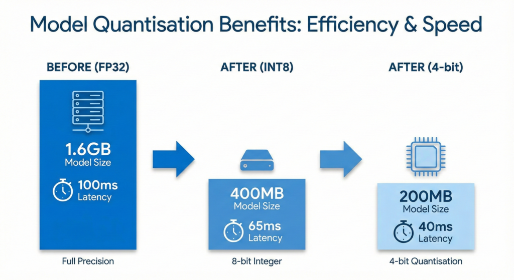
Post-training quantisation offers the fastest path to latency reduction without retraining. Converting weights from FP32 to INT8 typically yields 4x memory reduction and 1.5-6x inference speedup, depending on hardware support.

Advanced implementations achieve even better results. 4-bit quantisation with BitsAndBytes can reduce latency by 40% whilst maintaining 95% of original performance. For on-device deployment, sub-8-bit quantisation achieves 30% memory savings and 32% latency reduction compared to standard 8-bit approaches.

Mixed-precision quantisation provides optimal results. Encoders typically benefit from w8-a8 (8-bit weights and activations), whilst decoders can use w4-a16 for better memory-bandwidth utilisation. Hardware-aware quantisation tools like HAQ automate this optimisation by measuring actual latency during the search process.

Knowledge Distillation Strategies

Knowledge distillation transfers capabilities from larger, more accurate models to faster, more compact students. For ASR, dual-mode training proves particularly effective—training streaming and full-context models jointly with shared weights.

The technique achieves 2.6-5.3% relative error reduction on streaming models whilst simplifying deployment. You maintain a single model that adapts behaviour based on latency requirements, eliminating the complexity of managing separate streaming and batch systems.

Similarity-preserving distillation extends this further. Rather than matching output distributions, you align internal representations between teacher and student networks. This approach delivers better streaming accuracy, especially when combined with multi-decoder architectures that leverage CTC, RNN-T, and attention objectives simultaneously.

How Does Hardware Choice Impact ASR Latency?

Software optimisation only takes you so far. Hardware selection and deployment strategy fundamentally determine achievable latency, especially at scale.

GPU Acceleration with TensorRT

NVIDIA TensorRT delivers 12x acceleration over baseline implementations through kernel fusion, precision calibration, and layer optimisation. For production ASR systems, TensorRT optimisation is non-negotiable—it’s the difference between 5-second and sub-500ms inference.

Modern GPUs like the H100 provide transformer-optimised architectures specifically designed for attention operations. When properly configured with TensorRT, these achieve mean latencies around 50ms for ASR modules and 280ms for TTS synthesis, enabling true real-time voice transformation.

NVIDIA Riva packages this optimisation into a production-ready SDK. It handles the complexity of TensorRT integration, model serving through Triton, and automatic batching for optimal throughput. For enterprise deployments requiring hundreds of concurrent streams, Riva provides the infrastructure to maintain consistent sub-second latency.

Edge and On-Device Deployment

Edge deployment eliminates network latency entirely, crucial for applications demanding ultra-low response times. Apple’s Neural Engine exemplifies specialised NPU acceleration, with WhisperKit achieving 460ms latency and industry-leading 2.2% WER through aggressive model optimisation.

The optimisation required for edge deployment is substantial. WhisperKit compresses Whisper Large v3 Turbo from 1.6GB to 600MB using novel compression techniques whilst maintaining accuracy within 1% of the original. Streaming inference modifications enable the audio encoder to process incremental chunks rather than fixed 30-second windows.

For call centre applications, edge processing offers additional benefits: reduced cloud costs, improved privacy compliance, and resilience to network issues. However, you’ll need to carefully balance model size constraints against accuracy requirements for your specific use case.

Which Latency-Accuracy Trade-offs Should You Make?

Different applications demand different latency targets. Understanding these trade-offs helps you optimise effectively without over-engineering.

Latency Targets by Use Case

• Voice agents and AI assistants: Target 700-1500ms maximum latency. This range enables natural conversation flow whilst allowing aggressive optimisations. Accuracy degradation of less than 5% relative to batch processing is acceptable.
• Call centre transcription and captioning: Aim for 2-second latency as the sweet spot. This delivers only 1% accuracy degradation compared to batch processing whilst maintaining real-time context for agent assistance and quality monitoring.
• Legal and healthcare documentation: Accept 4-second latency to achieve accuracy equivalent to batch transcription. In these regulated environments, accuracy trumps speed, though you still benefit from streaming capabilities for workflow efficiency.

Most systems implement partial transcripts alongside final transcripts. Partials appear in under 500ms with 10-25% lower accuracy, providing immediate feedback whilst final transcripts refine the output. This dual-output approach satisfies both user experience and accuracy requirements.

Configurable Latency Parameters

Production ASR systems expose latency controls that balance speed against accuracy. The max_delay parameter determines how long the system waits after speech ends before returning final transcripts. Lower values (0.7-1.5s) suit conversational AI, whilst higher values (4s) optimise for accuracy-critical applications.

The max_delay_mode setting determines entity formatting behaviour. “Flexible” mode delays final transcripts until numbers, currencies, and dates are properly formatted, improving readability at the cost of variable latency. “Fixed” mode maintains strict latency guarantees but may sacrifice formatting accuracy.

I recommend starting with 2-second max_delay and flexible mode for most business applications. This configuration delivers excellent accuracy whilst maintaining perceptibly real-time response. You can then adjust based on actual user feedback and specific workflow requirements.

What Implementation Patterns Deliver Best Results?

Theory is valuable, but practical implementation determines success. These patterns emerge consistently in production systems achieving sub-second latency.

Concurrent Processing Architecture

Sequential processing creates unnecessary latency. Modern implementations use producer-consumer patterns to parallelise independent operations. ASR transcription, RAG retrieval, LLM generation, and TTS synthesis can partially overlap when properly orchestrated.

One effective architecture achieves 940ms average total latency by running components concurrently: ASR (50ms), retrieval (8ms negligible), LLM generation (670ms), and TTS synthesis (280ms). Without concurrency, these would sum to over 1 second, exceeding acceptable thresholds for interactive applications.

Time-to-first-token (TTFT) and time-to-first-audio (TTFA) become critical metrics. Users perceive responsiveness from initial output, not final completion. Streaming architectures that deliver partial results within 200-300ms feel responsive even when complete processing takes longer.

Voice Activity Detection Integration

Voice Activity Detection dramatically improves both latency and accuracy. By segmenting audio at natural silence points, you avoid processing long pauses that waste GPU cycles and introduce recognition errors.

WebSocket-based implementations combine VAD with streaming protocols for optimal results. The VAD component identifies speech boundaries, the WebSocket maintains bidirectional real-time communication, and the ASR engine processes only relevant audio segments. This approach achieves 300ms end-to-end latency in production environments.

For call centre applications, VAD serves dual purposes: optimising transcription performance and enabling utterance segmentation for speaker diarisation. This improves readability whilst reducing computational requirements compared to processing entire calls as single streams.

How Do You Measure and Monitor ASR Latency?

You can’t optimise what you don’t measure. Comprehensive latency monitoring requires tracking multiple metrics across the entire pipeline.

Real-Time Factor (RTF) Measurement

Real-Time Factor provides the fundamental performance metric for ASR systems. It’s calculated by dividing processing time by audio duration. An RTF of 0.6 means processing 10 seconds of speech takes 6 seconds—fast enough for offline processing but inadequate for real-time applications.

Target RTF below 1.0 for streaming applications, with sub-0.2 optimal for production systems. This 5x speed margin accommodates concurrent streams, variability in speech complexity, and system load fluctuations without degrading user experience.

Monitor RTF separately for encoder and decoder components. Encoders are typically activation-constrained (memory I/O dominated), whilst decoders are weight-constrained. This distinction guides optimisation strategy—quantise encoder activations aggressively, focus decoder optimisation on weight compression.

End-to-End Latency Tracking

RTF alone doesn’t capture user-perceived latency. You need end-to-end measurement from speech occurrence to transcript availability. The Deepgram methodology measures this as the difference between audio cursor and transcript cursor positions, accounting for word-level timestamps.

Implement detailed timing instrumentation at each pipeline stage. Record audio capture latency, model inference time, post-processing duration, network transit time, and redaction overhead separately. This granular visibility identifies optimisation bottlenecks and prevents premature optimisation of non-critical components.

For production monitoring, track latency percentiles (P50, P95, P99) rather than just averages. Tail latencies often degrade user experience more than average performance suggests. If P99 latency exceeds 2 seconds, investigate even when average latency appears acceptable.

What Are the Latest Advances in Low-Latency ASR?

The field evolves rapidly. Recent breakthroughs demonstrate what’s possible with aggressive optimisation and purpose-built architectures.

Conversational Models with Turn Detection

Traditional ASR treats transcription as isolated utterance processing. Conversational models like Deepgram’s Flux architecture build turn detection, natural interruption handling, and conversation understanding directly into the model.

These purpose-built systems achieve the same transcription accuracy as general models whilst delivering ultra-low latency specifically optimised for dialogue. Turn detection eliminates the need for external segmentation logic, reducing latency and simplifying deployment.

For call centres, this architectural shift proves transformative. Real-time sentiment analysis, agent coaching, and compliance monitoring become practical when transcription latency drops below perception thresholds and turn boundaries are automatically identified.

Domain-Specific Model Optimisation

General-purpose models sacrifice efficiency trying to handle every possible scenario. Domain-specific optimisation delivers superior latency by focusing on relevant vocabulary and acoustic conditions.

Healthcare implementations demonstrate this approach. Nova-3 Medical Streaming achieves clinical-grade accuracy for medical terminology whilst maintaining sub-second latency for live dictation and telehealth applications. The model understands medical context, eliminating the processing overhead of generic models attempting to disambiguate specialised terms.

For Indian languages, models like IndicConformer provide optimised implementations specifically targeting regional speech patterns and code-mixing. These deliver better accuracy at lower latency than general multilingual models by focusing computational resources on relevant linguistic features.

Conclusion: Building Your Low-Latency ASR System

Reducing latency in real-time speech recognition requires systematic optimisation across architecture, models, and hardware. Start by understanding your latency requirements—voice agents need sub-1.5s, call centres perform well at 2s, whilst documentation applications can accept 4s for maximum accuracy.

Focus optimisation efforts where they deliver maximum impact. Model inference accounts for 50-60% of latency, making architectural improvements and quantisation your highest-priority targets. GPU acceleration with TensorRT provides 12x speedups, whilst edge deployment eliminates network latency entirely for appropriate use cases.

Remember that latency optimisation trades off against accuracy, cost, and complexity. The goal isn’t achieving the absolute lowest latency possible—it’s delivering the optimal balance for your specific application and user requirements. Measure comprehensively, optimise systematically, and validate against real-world usage patterns.